Machine Learning Algorithms — Classification Tasks

Machine Learning Algorithms — Classification Task

scikit-learn: machine learning in Python — scikit-learn 1.7.2 documentation

Classification Task — Handwritten Digit Prediction

As a brief aside, let’s practice data visualization.

We can look at this dataset and try visualizing its first data point.

digits = datasets.load_digits()
X,y = digits.data,digits.target

print(X[0])
####
[ 0.  0.  5. 13.  9.  1.  0.  0.  0.  0. 13. 15. 10. 15.  5.  0.  0.  3.
 15.  2.  0. 11.  8.  0.  0.  4. 12.  0.  0.  8.  8.  0.  0.  5.  8.  0.
  0.  9.  8.  0.  0.  4. 11.  0.  1. 12.  7.  0.  0.  2. 14.  5. 10. 12.
  0.  0.  0.  0.  6. 13. 10.  0.  0.  0.]

It is a one-dimensional array of 64 values; use NumPy to reshape it into an 8×8 array.

digit_image =  np.reshape(X[0], (8,8))
print(digit_image)
print("数据形状"+digit_image.shape)

#### 
[[ 0.  0.  5. 13.  9.  1.  0.  0.]
 [ 0.  0. 13. 15. 10. 15.  5.  0.]
 [ 0.  3. 15.  2.  0. 11.  8.  0.]
 [ 0.  4. 12.  0.  0.  8.  8.  0.]
 [ 0.  5.  8.  0.  0.  9.  8.  0.]
 [ 0.  4. 11.  0.  1. 12.  7.  0.]
 [ 0.  2. 14.  5. 10. 12.  0.  0.]
 [ 0.  0.  6. 13. 10.  0.  0.  0.]]
(8, 8)

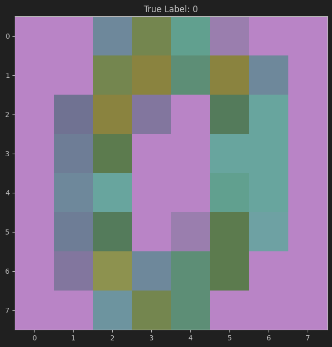
Visualize it directly with plt. Here, I used a colorful cmap to emphasize the visual appearance.

plt.figure(figsize=(8,8))
plt.imshow(digit_image, cmap=plt.cm.viridis, interpolation='nearest')
plt.title(f'True Label: {y[0]}')
plt.show()

The result is as follows. This dataset mainly maps handwritten data into a one-dimensional array.

Back to the main topic: what we are studying here is

from sklearn import datasets
from sklearn.linear_model import LogisticRegression
from sklearn.metrics import accuracy_score
from sklearn.model_selection import train_test_split

digits = datasets.load_digits()
X,y = digits.data,digits.target

# 划分训练集和测试集
X_train, X_test, y_train, y_test = train_test_split(X, y, test_size=0.3, random_state=42)

clf = LogisticRegression(max_iter=10000)
clf.fit(X_train, y_train)

y_pred = clf.predict(X_test)

print("预测结果", y_pred[:30])
print("真是结果", y_test[:30])
print(accuracy_score(y_test, y_pred))

'''
C:\Users\bx336\PycharmProjects\machine\.venv\Scripts\python.exe C:\Users\bx336\PycharmProjects\machine\start\1.py 
预测结果 [6 9 3 7 2 1 5 2 5 2 1 9 4 0 4 2 3 7 8 8 4 3 9 7 5 6 3 5 6 3]
真是结果 [6 9 3 7 2 1 5 2 5 2 1 9 4 0 4 2 3 7 8 8 4 3 9 7 5 6 3 5 6 3]
0.9685185185185186
'''

One detail I think is important is splitting the data.

One part of a dataset is used for training, and another part is used for testing.

X_train, X_test, y_train, y_test = train_test_split(X, y, test_size=0.3, random_state=42)

This is actually easy to understand; just look at the specific parameters.

• test_size means the test set accounts for 20% of the total data, and the training set makes up the remaining 80%.
• random_state=42 is the random seed.

The last item is accuracy_score.

from sklearn.metrics import accuracy_score

y_true = [0, 1, 2, 2, 0]    # 真实标签
y_pred = [0, 0, 2, 2, 0]    # 模型预测

acc = accuracy_score(y_true, y_pred)
print(acc)

Accuracy = number of correctly predicted samples / total number of samples.